Reinforcement Learning [Part 0]
- 2147 words
- 11 min
You might be tired of hearing of it by now, but it's impossible to start a blog series on Reinforcement Learning without mentioning the game of Go in the first 5 lines.
It all started in May 2016: AlphaGo, a computer program developed by Google, won 4 Go games (in a series of 5) against Lee Sedol, the current World Champion. (link)
Defining the event as "an historic achievement" is an understatement: the game of Go proved to be way more difficult for machines than chess - too many possible configurations of the game board, an impossible task to solve with brute force alone.
Nonetheless we managed to find our way in this huge maze of possibilities, setting a new milestone for AI way sooner than expected. How did Google accomplish it?
Combining Deep Learning and Reinforcement Learning in one of the hottest AI labs in the world - DeepMind, bought by Google in 2014 for 400 millions of dollars.
Unsatisfied, they improved on their own results releasing AlphaGoZero in October 2017 (link) and AlphaZero in December 2017 (link) - quick spoiler: AlphaGo used, to a certain extent, some human-taught heuristics; his children with superpowers dispose of everything human-related.
Now, a much needed warning: if you expect me to start explaining how AlphaGo works, suggesting cool but vague analogies with human learning without providing any solid connection between consecutive steps.... Well, you came to the wrong blog.
It will probably take me 6 or more posts to even start touching the interesting and nuanced ways found by researchers to combine Deep Learning and Reinforcement Learning before AlphaGo came to life.
The reason is dead simple: most of us have no first-hand experience of Reinforcement Learning, apart from popular news articles and a quick skim of related Arxiv papers without a serious learning intent. Even worse, we have no idea of the underlying mathematical model - Markov Decision Processes (MDPs).
I am a fan of the old-fashioned idea of building a house from the ground up: this is but the preface of a long series of blog posts meant to introduce Reinforcement Learning starting from scratch, taking the proper time to learn the basics concepts without cutting corners or shying away from the required math.
I know of no other way to properly master a subject, and you should understand that we are embarking on this trip together: think of this series as the journal of a curious Machine Learning practitionier who wants to learn and master Reinforcement Learning.
If you share my style, be my guest - suggestions, critiques and contributions are welcome.
If you struggle with my approach, my apologies - I hope I have not wasted too much of your time, you can still flee in your world of catchy Machine Learning headlines.

Well, we can cut short on pleasantries and finally get started!
Basic Ideas
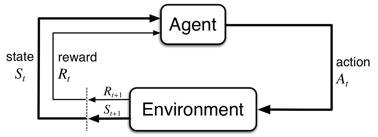
Many real world problems can be formulated as the interaction between an agent and an environment.
The agent interacts with the environment performing actions trying to achieve a certain goal. Every action might cause a change in the environment state.
Examples are abundant.
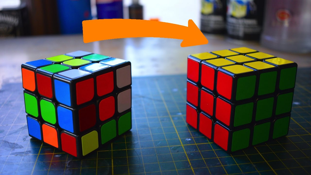
We might consider, for instance, a human trying to solve a Rubik cube as an agent (the player) interacting with its environment (the cube) through a specific set of actions (cube moves) in order to achieve its final goal (solved cube).

Agent, environment and state are very flexible concepts - we should not let realism be our first concern and, depending on the goal our agent is supposed to achieve, we have to choose the most appropriate way to model each one of them.
If our goal in the Rubik cube problem is to find the shortest sequence of action leading to a solution then we can simply model the environment state as an array of 6 3x3 matrices, one for each face of the cube, where each entry corresponds to the first letter of the respective tile color.
If our aim, instead, is to find the best hand technique in order to physically solve the cube in the shortest amount of time we do have to retain more informations: the physical position of the cube in the space, its internal mechanism, etc.
Slightly different aims, substantially different formulations.
Let's denote by $\mathcal{S}$ the set of possible states of our system.
For the easiest formulation of the Rubik cube problem we have
$$ \mathcal{S} = \{r, b, g, o, w, y\}^{6\times (3\times 3)} $$
We shall denote by $\mathcal{A}(s)$ the set actions available to the agent if the current system state is $s\in\mathcal{S}$ - I won't formalize the action space in the case of the Rubik cube. Rubik cubes are cute, simple and everyone knows them but I don't care enough about them to break the sweat - don't take offense Rubik pros.
If the set actions does not depend on the current system state, as in our current example, we will use $\mathcal{A}$ as a short-hand notation.
We will always assume, unless otherwise specified, that time is discrete: the agent has the chance to perform an action for every $t\in\mathbb{N}=\{1,2,\dots\}$.
The initial state of the system will be denoted by $S_1\in\mathcal{S}$.
The agent evaluates the situation and reacts accordingly - its action will be denoted by $A_1$.
Iterating this procedure we obtain the trajectory or history of our simulation:
$$\begin{equation} S_1, \, A_1, \, S_2, \, A_2, \, S_3, \, \dots \end{equation}$$
The trajectory is a perfect description of what is happening, but does not provide any information concerning the goal of the agent. How is it supposed to learn the best way to achieve its purpose?
We need to introduce some kind of feedback, going from the environment to the agent, whose purpose is to help the agent realize the connection between its current action and the achievement of its ultimate goal.
In Reinforcement Learning this takes the form of a scalar signal, called reward.

After every action $A_t$ the agent receives a reward $R_{t+1}$ - a real number, either positive or negative:
$$\begin{equation} S_1, \,A_1, \,R_2, \,S_2, \,A_2, \,R_3, \,S_3, \,\dots \end{equation}$$
The aim of the agent is to maximize the total sum of the rewards it is going to collect.
In our Rubik cube example, for instance, we might provide the agent with a $-1$ reward if the state following its latest action is not a solved cube while we provide a $+1$ reward if its latest action solves the cube.
Does this actually point the agent in the right direction?
Yes! The expected total reward of our agent is
$$\begin{equation} \sum_{t=1}^T R_{t+1} = -(T - 1) +1 = -T + 2 \end{equation}$$
where $T$ is the number of moves our agent needs to reach a solution. The lower $T$, the higher the expected total reward - we are pushing our agent to do better with respect to the goal we have defined!
The common principle underlying Reinforcement Learning techniques is the so-called reward hypothesis:
That all of what we mean by goals and purposes can be well thought of as maximization of the expected value of the cumulative sum of a received scalar signal (called reward).
The extent to which this hypothesis can be accepted is debatable - designing a proper system of rewards is not always easy as well as understanding if those rewards do actually point the agent in the desired direction. Nonetheless we shall accept it as a working hypothesis and reason in the framework it provides.
Markov Decision Processes (MDPs)
Most of the systems we are actually interested in are unfortunately a little more messy than a Rubik cube: for instance, the evolution of the system might be stochastic instead of deterministic. The same applies to rewards - a specific pair of state and action might lead to different rewards, each one with its own probability.
We need to take all these possibilities into account and provide a sufficiently general formalism to reason about them.
This is why we approach a Reinforcement Learning system as a stochastic process - a sequence of random variables.
What random variables?
The sequence of states, actions and rewards we have just defined! $S_1$, $A_1$, $R_2$, $S_2$ and so on.
The environment is fully known once we have properly specified:
- the probability of receiving a reward
$r$at time$t+1$knowing the system history up to that moment:$$\begin{equation} \mathbb{P}(R_{t+1}=r \, | \, A_{t}=a_t, \,S_{t}=s_t,\, A_{t-1}=a_{t-1}, \, \dots, \, S_1=s_1) \end{equation}$$for each$t\in\mathbb{N}$, for all$s_t, \, s_{t-1}, \, \dots, \, s_1\in\mathcal{S}$and for all$a_i\in\mathcal{A}(s_i)$,$i\in\{1,\dots, t\}$; - the probability of ending up in state
$s$at time$t+1$knowing the system history up to that moment:$$\begin{equation} \mathbb{P}(S_{t+1}=s \, | \, A_{t}=a_t, \,S_{t}=s-t,\, A_{t-1}=a_{t-1}, \, \dots, \, S_1=s_1) \end{equation}$$for each$t\in\mathbb{N}$, for all$s_t, \, s_{t-1}, \, \dots, \, s_1\in\mathcal{S}$and for all$a_i\in\mathcal{A}(s_i)$,$i\in\{1,\dots, t\}$.
We will always assume that rewards are markovian - they only depend on the latest pair of state-action. Formally:
$$\begin{equation} \mathbb{P}(R_{t+1}=r \, | \, A_{t}=a_t, \,S_{t}=s_t,\, \dots, \, S_1=s_1) = \mathbb{P}(R_{t+1}=r \, | \, A_{t}=a_t, \,S_{t}=s_t) \end{equation}$$
Most of the times we will assume markovianity also for the state random variable, $S_t$ - in this case the mathematical formulation of a Reinforcement Learning problem takes the name of Markov Decision Process (MDP).
We are going to study them in depth during the rest of our journey.
As we said, the environment is responsible for the behaviour of states and rewards. The agent, instead, is fully determined by the probability of taking action $a$ at time $t$ knowing the system history up to that moment:
$$\begin{equation} \mathbb{P}(A_{t}=a \, | \, S_{t},\, A_{t-1}, \, \dots, \, S_1) \end{equation}$$
for each $t\in\mathbb{N}$.
A complete specification of the agent behaviour is usually called policy - the part we want to optimize, the heart of the problem we want to solve.
These are all the ingredients we need.
As in a true kitchen, we have to find out the inner relationships between them, uncovering the underlying structure and using their properties for our own purposes.
For a preface I'd say we have covered enough - the next post will delve deeper into the definition of policy, that we have barely touched, as well as formalizing properly the notion of expected cumulative return, which lays at the center of the reward hypothesis we stated before.
We shall use the first 2 or 3 posts to lay down the theory underlying Reinforcement Learning, but we will provide properly coded examples as soon as we touch the first useful algorithms.
Bear with me during these first math-heavy episodes - your perseverance will pay off sooner than you expect.
References & Prerequisites

Most of this series will be freely based on:
- "Reinforcement Learning: an introduction" by Sutton and Barto (freely downloadable here);
- "Markov Decision Processes" by Puterman (2005 edition).
Sutton's book is a gentle intro, quite practical in spirit, while Puterman's book is a mathematical essay on Markov Decision Processes - we'll try to get the best out of both of them, properly shifting our focus depending on the topic at hand.
Books are extremely useful - use them as a truth source every time a passage in my posts leaves you lost and in despair (as well as pointing me out what you found confusing or unclear!).
I won't assume any previous knowledge apart from basic calculus and probability theory. I'll try to provide links and easy references every time I mention a more advanced topic. Once again, if a certain notation or passage confuses you don't hesitate to leave a comment asking for clarifications - everyone has been there before!